# xtick이 항상 10개 출력되도록 - 아래 x축 label step = len(kor_vs_cur) // 10 plt.xticks(kor_vs_cur.index[::step])
plt.show()
상관계수 확인 - KOSPI
1 2 3 4 5 6 7 8 9 10
#상관계수 확인 - "KOSPI" print("KOSPI vs KOSDAQ : {}".format(np.corrcoef(kor_vs_cur["kospi"], kor_vs_cur["kosdaq"])[0, 1])) print("KOSPI vs USDKRW : {}".format(np.corrcoef(kor_vs_cur["kospi"], kor_vs_cur["usd"])[0, 1])) print("KOSPI vs CNYKRW : {}".format(np.corrcoef(kor_vs_cur["kospi"], kor_vs_cur["cny"])[0, 1])) print("KOSPI vs JPYKRW : {}".format(np.corrcoef(kor_vs_cur["kospi"], kor_vs_cur["jpy"])[0, 1])) print("KOSPI vs EURKRW : {}".format(np.corrcoef(kor_vs_cur["kospi"], kor_vs_cur["eur"])[0, 1])) print("KOSPI vs INRKRW : {}".format(np.corrcoef(kor_vs_cur["kospi"], kor_vs_cur["inr"])[0, 1])) print("KOSPI vs GBPKRW : {}".format(np.corrcoef(kor_vs_cur["kospi"], kor_vs_cur["gbp"])[0, 1])) print("KOSPI vs BRLKRW : {}".format(np.corrcoef(kor_vs_cur["kospi"], kor_vs_cur["brl"])[0, 1])) print("KOSPI vs CADKRW : {}".format(np.corrcoef(kor_vs_cur["kospi"], kor_vs_cur["cad"])[0, 1]))
KOSPI vs KOSDAQ : 0.8689701457832764
KOSPI vs USDKRW : -0.7474526625164396
KOSPI vs CNYKRW : -0.8299251745227267
KOSPI vs JPYKRW : -0.6105987487442344
KOSPI vs EURKRW : -0.2986694402889244
KOSPI vs INRKRW : -0.09305307626089275
KOSPI vs GBPKRW : 0.4807979987407145
KOSPI vs BRLKRW : 0.267607616153946
KOSPI vs CADKRW : 0.6836357941585803
# xtick이 항상 10개 출력되도록 - 아래 x축 label step = len(kor_vs_cur) // 10 plt.xticks(kor_vs_cur.index[::step])
plt.show()
상관계수 확인 - “KOSDAQ”
1 2 3 4 5 6 7 8 9
print("KOSDAQ vs KOSDAQ : {}".format(np.corrcoef(kor_vs_cur["kosdaq"], kor_vs_cur["kospi"])[0, 1])) print("KOSDAQ vs USDKRW : {}".format(np.corrcoef(kor_vs_cur["kosdaq"], kor_vs_cur["usd"])[0, 1])) print("KOSDAQ vs CNYKRW : {}".format(np.corrcoef(kor_vs_cur["kosdaq"], kor_vs_cur["cny"])[0, 1])) print("KOSDAQ vs JPYKRW : {}".format(np.corrcoef(kor_vs_cur["kosdaq"], kor_vs_cur["jpy"])[0, 1])) print("KOSDAQ vs EURKRW : {}".format(np.corrcoef(kor_vs_cur["kosdaq"], kor_vs_cur["eur"])[0, 1])) print("KOSDAQ vs INRKRW : {}".format(np.corrcoef(kor_vs_cur["kosdaq"], kor_vs_cur["inr"])[0, 1])) print("KOSDAQ vs GBPKRW : {}".format(np.corrcoef(kor_vs_cur["kosdaq"], kor_vs_cur["gbp"])[0, 1])) print("KOSDAQ vs BRLKRW : {}".format(np.corrcoef(kor_vs_cur["kosdaq"], kor_vs_cur["brl"])[0, 1])) print("KOSDAQ vs CADKRW : {}".format(np.corrcoef(kor_vs_cur["kosdaq"], kor_vs_cur["cad"])[0, 1]))
KOSDAQ vs KOSDAQ : 0.8689701457832764
KOSDAQ vs USDKRW : -0.4560788590919353
KOSDAQ vs CNYKRW : -0.7171914703642415
KOSDAQ vs JPYKRW : -0.24811709011626565
KOSDAQ vs EURKRW : -0.019148376695966446
KOSDAQ vs INRKRW : -0.3900569760483904
KOSDAQ vs GBPKRW : 0.21872439893983708
KOSDAQ vs BRLKRW : -0.21073197177622852
KOSDAQ vs CADKRW : 0.49393118449595613
# xtick이 항상 10개 출력되도록 - 아래 x축 label step = len(kor_vs_cur) // 10 plt.xticks(kor_vs_cur.index[::step])
plt.show()
추가 상관계수 확인 - “USD”
확실히 KOSPI나 KOSDAQ과 비교했을 때 전체적으로 상관계수들이 비교적 높다
USD 상관계수 절대값 0.4 미만 = 2개
KOSPI 상관계수 절대값 0.4 미만 = 3개
KOSDAQ 상관계수 절대값 0.4 미만 = 5개
달러의 움직임이 전세계에 영향을 미친다는 것을 알 수 있다.
1 2 3 4 5 6 7 8 9
print("USD vs KOSPI : {}".format(np.corrcoef(kor_vs_cur["usd"], kor_vs_cur["kospi"])[0, 1])) print("USD vs KOSDAQ : {}".format(np.corrcoef(kor_vs_cur["usd"], kor_vs_cur["kosdaq"])[0, 1])) print("USD vs CNYKRW : {}".format(np.corrcoef(kor_vs_cur["usd"], kor_vs_cur["cny"])[0, 1])) print("USD vs JPYKRW : {}".format(np.corrcoef(kor_vs_cur["usd"], kor_vs_cur["jpy"])[0, 1])) print("USD vs EURKRW : {}".format(np.corrcoef(kor_vs_cur["usd"], kor_vs_cur["eur"])[0, 1])) print("USD vs INRKRW : {}".format(np.corrcoef(kor_vs_cur["usd"], kor_vs_cur["inr"])[0, 1])) print("USD vs GBPKRW : {}".format(np.corrcoef(kor_vs_cur["usd"], kor_vs_cur["gbp"])[0, 1])) print("USD vs BRLKRW : {}".format(np.corrcoef(kor_vs_cur["usd"], kor_vs_cur["brl"])[0, 1])) print("USD vs CADKRW : {}".format(np.corrcoef(kor_vs_cur["usd"], kor_vs_cur["cad"])[0, 1]))
USD vs KOSPI : -0.7474526625164396
USD vs KOSDAQ : -0.45607885909193524
USD vs CNYKRW : 0.8717121292793995
USD vs JPYKRW : 0.7276336988139611
USD vs EURKRW : 0.47570951394792504
USD vs INRKRW : 0.13242540153627583
USD vs GBPKRW : -0.45775893555193975
USD vs BRLKRW : -0.4943384202903821
USD vs CADKRW : -0.3276584506393807
# df.count() does not include NaN values # remove Id and the features with 30% or less NaN values df2 = df[[column for column in df if df[column].count() / len(df) >= 0.3]] del df2['Id'] print("List of dropped columns:", end=" ") for c in df.columns: if c notin df2.columns: print(c, end=", ")
print('\n') df = df2
List of dropped columns: Id, Alley, PoolQC, Fence, MiscFeature,
1 2 3 4
# the distribution of the housing price print(df['SalePrice'].describe()) plt.figure(figsize=(9, 8)) sns.distplot(df['SalePrice'], color='g', bins=100, hist_kws={'alpha': 0.4});
count 1460.000000
mean 180921.195890
std 79442.502883
min 34900.000000
25% 129975.000000
50% 163000.000000
75% 214000.000000
max 755000.000000
Name: SalePrice, dtype: float64
From the above graph, it can be deduced that there are outliers existing above $500,000. These outliers will be deleted to get a normal distribution of the independent variabl ('SalePrice') for machine learning <= (not sure what this means)
“Features such as 1stFlrSF, TotalBsmtSF, LotFrontage, GrLiveArea… seems to share a similar distribution to the one we have with SalePrice. Lets see if we can find new clues later.”
At this point, I suddenly came to wonder what are we trying to find through all this process? Why does it seem like the SalePrice is the center of the whole thing.
1 2 3
df_num_corr = df_num.corr()['SalePrice'][:-1] # -1 because the last row is SalePrice golden_features_list = df_num_corr[abs(df_num_corr) > 0.5].sort_values(ascending=False) print("The following are the top {} strongly correlated values with SalePrice:\n{}".format(len(golden_features_list), golden_features_list))
The following are the top 10 strongly correlated values with SalePrice:
OverallQual 0.790982
GrLivArea 0.708624
GarageCars 0.640409
GarageArea 0.623431
TotalBsmtSF 0.613581
1stFlrSF 0.605852
FullBath 0.560664
TotRmsAbvGrd 0.533723
YearBuilt 0.522897
YearRemodAdd 0.507101
Name: SalePrice, dtype: float64
From the table above, we now know which data has the strongest relationship with the SalePrice. But, this data is still incomplete as the outliers still exist in the dataset.
To get rid of the outliers the following measures can be taken:
1 2 3
1. Plot the numerical features and see which ones have very few or explainable outliers
2. Remove the outliers from these features and see which one can have a good correlation without their outliers
NOTE 1
Correlation by itself does not always explain the relationship between data
Plotting data could lead to new insights
THEREFORE ALWAYS VISUALIZE THE DATA
NOTE 2
Through the correlation value,the curvilinear relationship cannot be deduced.
SO ALWAYS VISUALIZE THE DATA IN NUMEROUS WAYS TO GET MORE INSIGHTS
1
For example, relationships such as curvilinear relationship cannot be guessed just by looking at the correlation value so lets take the features we excluded from our correlation table and plot them to see if they show some kind of pattern.
Not sure yet what features were excluded from the correlation table.
1
2
3
4
5
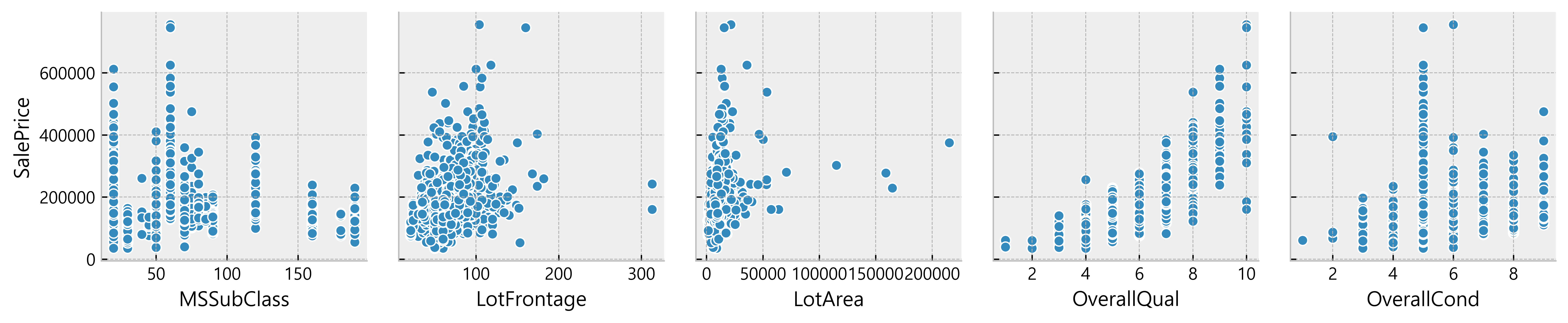
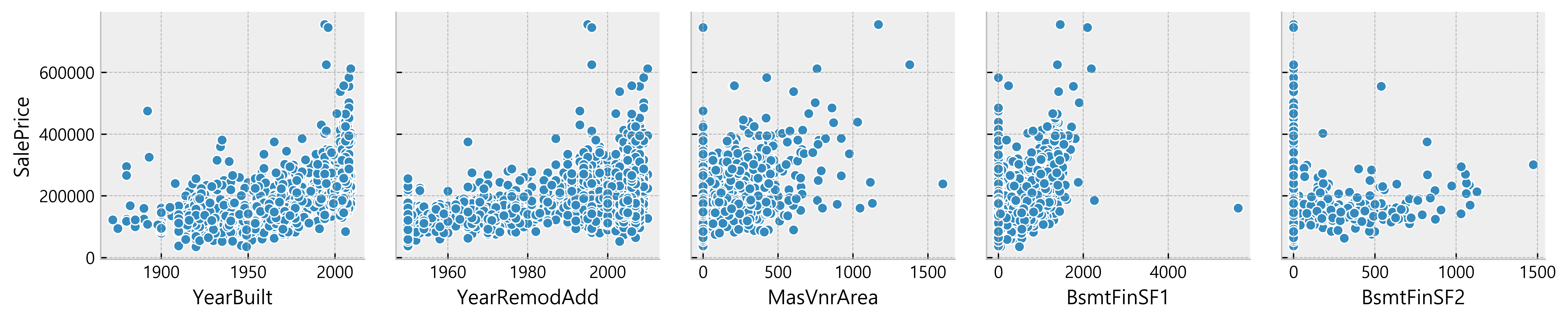
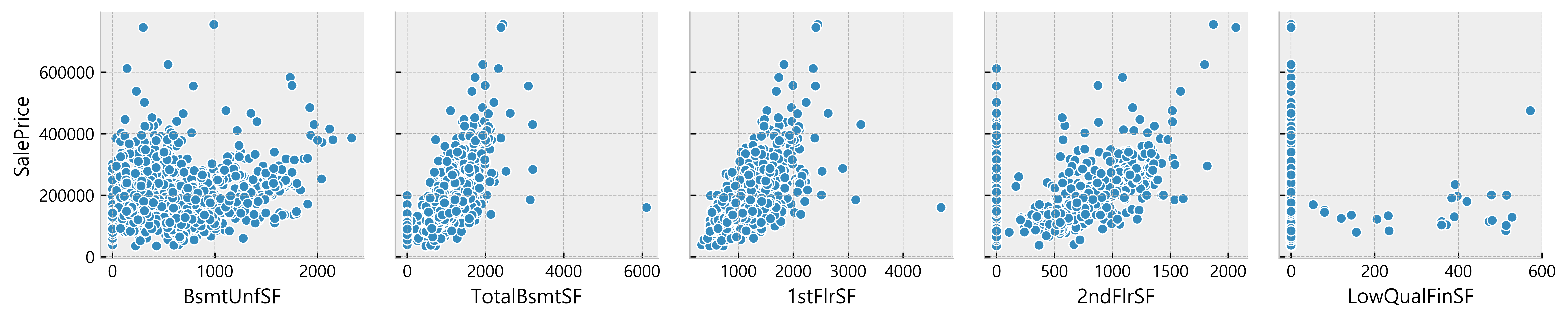
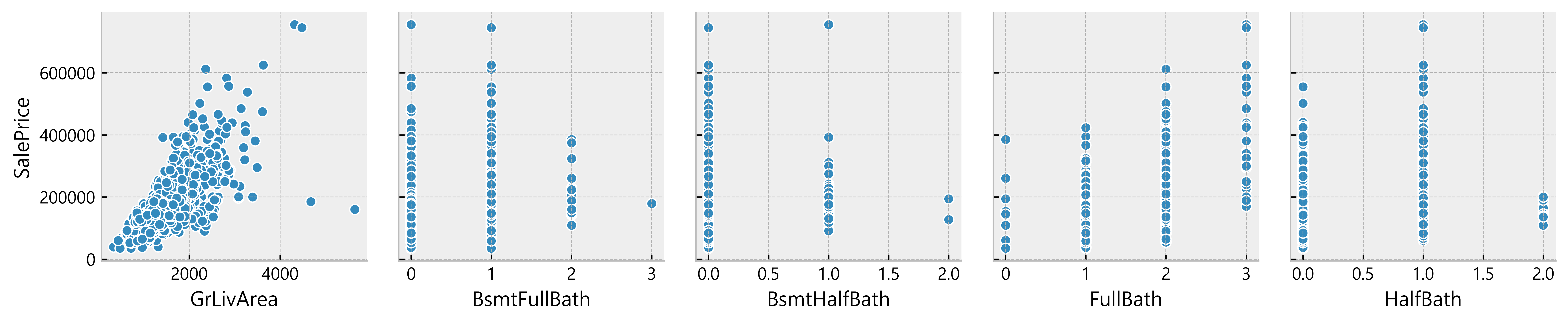
for i in range(0, len(df_num.columns), 5): sns.pairplot(data=df_num, x_vars=df_num.columns[i:i+5], y_vars=['SalePrice'] )
Deduction:
- Many data seem to have a linear relationship with the SalePrice
- A lot of data points are located on x = 0
Possible indication of absence of such features in the house)
More Data Cleaning
Removal of 0 values and repeat the process of finding correlated values
1 2 3 4 5 6 7 8 9 10 11 12 13 14
import operator
individual_features_df = [] for i in range(0, len(df_num.columns) - 1): # -1 because the last column is SalePrice tmpDf = df_num[[df_num.columns[i], 'SalePrice']] tmpDf = tmpDf[tmpDf[df_num.columns[i]] != 0] individual_features_df.append(tmpDf) all_correlations = {feature.columns[0]: feature.corr()['SalePrice'][0] for feature in individual_features_df} all_correlations = sorted(all_correlations.items(), key=operator.itemgetter(1))
for (key, value) in all_correlations: print("{:>15}: {:>15}".format(key, value))
The most strongly correlated values are as follows in the golden_features_list.
1 2
golden_features_list = [key for key, value in all_correlations if abs(value) >= 0.5] print("Following are the top {} strongly correlated values with SalePrice:\n{}".format(len(golden_features_list), golden_features_list))
Following are the top 11 strongly correlated values with SalePrice:
['YearRemodAdd', 'YearBuilt', 'TotRmsAbvGrd', 'FullBath', '1stFlrSF', 'GarageArea', 'TotalBsmtSF', 'GarageCars', '2ndFlrSF', 'GrLivArea', 'OverallQual']
for i, ax in enumerate(fig.axes): if i < len(features_to_analyse) - 1: sns.regplot(x = features_to_analyse[i], y='SalePrice', data=df[features_to_analyse], ax=ax)
We can see that features such as TotalBsmtSF, 1stFlrSF, GrLivArea have a big spread but I cannot tell what insights this information gives us
C -> Q (Categorical to Quantitative Relationship)
1 2 3 4
# quantitative_features_list[:-1] as the last column is SalePrice and we want to keep it categorical_features = [a for a in quantitative_features_list[:-1] + df.columns.tolist() if (a notin quantitative_features_list[:-1]) or (a notin df.columns.tolist())] df_categ = df[categorical_features] df_categ.head()
MSSubClass
MSZoning
Street
LotShape
LandContour
Utilities
LotConfig
LandSlope
Neighborhood
Condition1
...
GarageYrBlt
GarageFinish
GarageQual
GarageCond
PavedDrive
MoSold
YrSold
SaleType
SaleCondition
SalePrice
0
60
RL
Pave
Reg
Lvl
AllPub
Inside
Gtl
CollgCr
Norm
...
2003.0
RFn
TA
TA
Y
2
2008
WD
Normal
208500
1
20
RL
Pave
Reg
Lvl
AllPub
FR2
Gtl
Veenker
Feedr
...
1976.0
RFn
TA
TA
Y
5
2007
WD
Normal
181500
2
60
RL
Pave
IR1
Lvl
AllPub
Inside
Gtl
CollgCr
Norm
...
2001.0
RFn
TA
TA
Y
9
2008
WD
Normal
223500
3
70
RL
Pave
IR1
Lvl
AllPub
Corner
Gtl
Crawfor
Norm
...
1998.0
Unf
TA
TA
Y
2
2006
WD
Abnorml
140000
4
60
RL
Pave
IR1
Lvl
AllPub
FR2
Gtl
NoRidge
Norm
...
2000.0
RFn
TA
TA
Y
12
2008
WD
Normal
250000
5 rows × 49 columns
non-numerical features
1
2
df_not_num = df_categ.select_dtypes(include = ['O']) # Object(O)
print('There are {} non numerical features including:\n{}'.format(len(df_not_num.columns), df_not_num.columns.tolist()))
“Looking at these features we can see that a lot of them are of the type Object(O). In our data transformation notebook we could use Pandas categorical functions (equivalent to R’s factor) to shape our data in a way that would be interpretable for our machine learning algorithm. ExterQual for instace could be transformed to an ordered categorical object.”
Definitely need more study on this especially on the transformation of data
for i, ax in enumerate(fig.axes): if i < len(df_not_num.columns): ax.set_xticklabels(ax.xaxis.get_majorticklabels(), rotation=45) sns.countplot(x=df_not_num.columns[i], alpha=0.7, data=df_not_num, ax=ax) fig.tight_layout()
Deduction
Some categories are predominant for some features e.g. Utilities, Heating, etc.
Welcome to Hexo! This is your very first post. Check documentation for more info. If you get any problems when using Hexo, you can find the answer in troubleshooting or you can ask me on GitHub.